Overview

In this lab, you:

• Deal with late data.
• Deal with malformed data by:
• Writing a composite transform for more modular code.
• Writing a transform that emits multiple outputs of different types.
• Collecting malformed data and writing it to a location where it can be examined.

The end of the previous lab introduces one sort of challenge that real-time pipelines must contend with: the gap between when events transpire and when they are processed, also known as lag. This lab introduces Apache Beam concepts that allow pipeline creators to specify how their pipelines should deal with lag in a formal way.

But lag isn’t the only sort of problem that pipelines are likely to encounter in a streaming context: whenever input comes from outside the system, there is always the possibility that it will be malformed in some way. This lab also introduces techniques that can be used to deal with such inputs.

The final pipeline in this lab resembles the picture below. Note that it contains a branch.

Setup and requirements

Before you click the Start Lab button

Note: Read these instructions.

Labs are timed and you cannot pause them. The timer, which starts when you click Start Lab, shows how long Google Cloud resources will be made available to you.

This Qwiklabs hands-on lab lets you do the lab activities yourself in a real cloud environment, not in a simulation or demo environment. It does so by giving you new, temporary credentials that you use to sign in and access Google Cloud for the duration of the lab.

What you need

To complete this lab, you need:

• Access to a standard internet browser (Chrome browser recommended).
• Time to complete the lab.

Note: If you already have your own personal Google Cloud account or project, do not use it for this lab. Note: If you are using a Pixelbook, open an Incognito window to run this lab.

How to start your lab and sign in to the Console

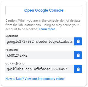
1. Click the Start Lab button. If you need to pay for the lab, a pop-up opens for you to select your payment method. On the left is a panel populated with the temporary credentials that you must use for this lab.

   

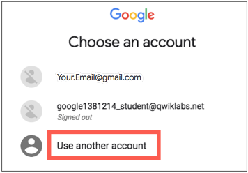
2. Copy the username, and then click Open Google Console. The lab spins up resources, and then opens another tab that shows the Choose an account page.

   Note: Open the tabs in separate windows, side-by-side.

3. On the Choose an account page, click Use Another Account. The Sign in page opens.

   

4. Paste the username that you copied from the Connection Details panel. Then copy and paste the password.

Note: You must use the credentials from the Connection Details panel. Do not use your Google Cloud Skills Boost credentials. If you have your own Google Cloud account, do not use it for this lab (avoids incurring charges).

5. Click through the subsequent pages:

• Accept the terms and conditions.
• Do not add recovery options or two-factor authentication (because this is a temporary account).
• Do not sign up for free trials.

After a few moments, the Cloud console opens in this tab.

Note: You can view the menu with a list of Google Cloud Products and Services by clicking the Navigation menu at the top-left.

Workbench Instances development environment setup

For this lab, you will be running all commands in a terminal from your Instance notebook.

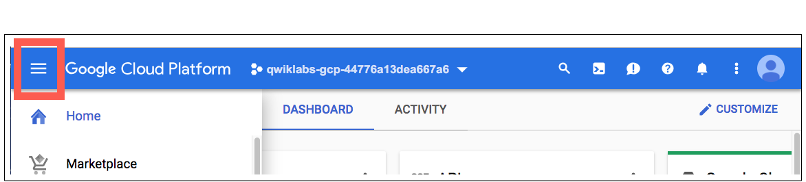
1. In the Google Cloud console, from the Navigation menu (), select Vertex AI > Dashboard.

2. Click Enable All Recommended APIs.

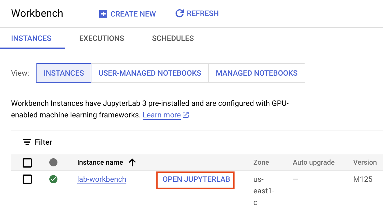
3. In the Navigation menu, click Workbench.

   At the top of the Workbench page, ensure you are in the Instances view.

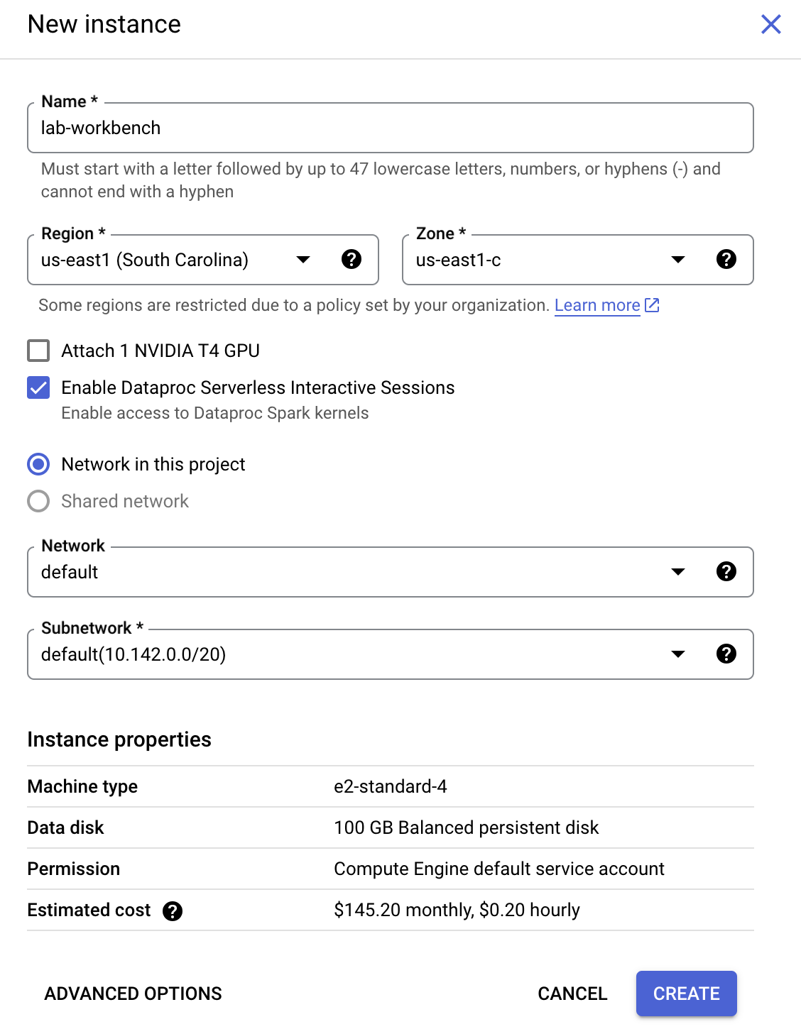
4. Click Create New.

5. Configure the Instance:

   • Name: lab-workbench
   • Region: Set the region to
   • Zone: Set the zone to
   • Advanced Options (Optional): If needed, click "Advanced Options" for further customization (e.g., machine type, disk size).

6. Click Create.

This will take a few minutes to create the instance. A green checkmark will appear next to its name when it's ready.

7. Click Open Jupyterlab next to the instance name to launch the JupyterLab interface. This will open a new tab in your browser.

8. Next, click Terminal. This will open up a terminal where you can run all the commands in this lab.

Download Code Repository

Next you will download a code repository for use in this lab.

1. In the terminal you just opened, enter the following:

git clone https://github.com/GoogleCloudPlatform/training-data-analyst cd /home/jupyter/training-data-analyst/quests/dataflow_python/

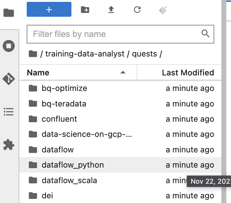
2. On the left panel of your notebook environment, in the file browser, you will notice the training-data-analyst repo added.

3. Navigate into the cloned repo /training-data-analyst/quests/dataflow_python/. You will see a folder for each lab, which is further divided into a lab sub-folder with code to be completed by you, and a solution sub-folder with a fully workable example to reference if you get stuck.

Note: To open a file for editing purposes, simply navigate to the file and click on it. This will open the file, where you can add or modify code.

Click Check my progress to verify the objective. Create notebook instance and clone course repo

Lab part 1: Dealing with late data

In the previous labs, you wrote code that divided elements by event time into windows of fixed width, using code that looked like the following:

parsed_msgs | "WindowByMinute" >> beam.WindowInto(beam.window.FixedWindows(window_duration)) | "CountPerMinute" >> beam.CombineGlobally(CountCombineFn()).without_defaults()

However, as you saw at the end of the last non-SQL lab, streams of data often have lag. Lag is problematic when windowing using event time (as opposed to processing time) because it introduces uncertainty: have all of the events for a particular point in event time actually arrived, or haven’t they?

Clearly, in order to output results, the pipeline you wrote needed to make a decision in this respect. It did so using a concept called a watermark. A watermark is the system’s heuristic-based notion of when all data up to a certain point in event time can be expected to have arrived in the pipeline. Once the watermark progresses past the end of a window, any further element that arrives with a timestamp in that window is considered late data and is simply dropped. So, the default windowing behavior is to emit a single, hopefully complete result when the system is confident that it has all of the data.

Apache Beam uses a number of heuristics to make an educated guess about what the watermark is. However, these are still heuristics. More to the point, those heuristics are general-purpose and are not suitable for all use cases. Instead of using general-purpose heuristics, pipeline designers need to thoughtfully consider the following questions in order to determine what tradeoffs are appropriate:

• Completeness: How important is it to have all of your data before you compute your result?
• Latency: How long do you want to wait for data? For example, do you wait until you think you have all data, or do you process data as it arrives?
• Cost: How much compute power and money are you willing to spend to lower the latency?

Armed with those answers, it’s possible to use Apache Beam’s formalisms to write code that makes the right tradeoff.

Allowed lateness

Allowed lateness controls how long a window should retain its state; once the watermark reaches the end of the allowed lateness period, all state is dropped. While it would be great to be able to keep all of our persistent state around until the end of time, in reality, when dealing with an unbounded data source, it’s often not practical to keep a given window's state indefinitely; we’ll eventually run out of disk space.

As a result, any real-world, out-of-order processing system needs to provide some way to bound the lifetimes of the windows it’s processing. A clean and concise way of doing this is by defining a horizon on the allowed lateness within the system, i.e. placing a bound on how late any given record may be (relative to the watermark) for the system to bother processing it; any data that arrives after this horizon is simply dropped. Once you’ve bounded how late individual data may be, you’ve also established precisely how long the state for windows must be kept around: until the watermark exceeds the lateness horizon for the end of the window.

Task 1. Prepare the environment

As in the prior labs, the first step is to generate data for the pipeline to process. You will open the lab environment and generate the data as before:

Open the appropriate lab

• In the terminal in your IDE, run the following commands to change to the directory you will use for this lab:

# Change directory into the lab cd 7_Advanced_Streaming_Analytics/lab export BASE_DIR=$(pwd)

Setting up virtual environment and dependencies

Before you can begin editing the actual pipeline code, you need to ensure you have installed the necessary dependencies.

1. Execute the following to create a virtual environment for your work in this lab:

sudo apt-get update && sudo apt-get install -y python3-venv ## Create and activate virtual environment python3 -m venv df-env source df-env/bin/activate

2. Next, install the packages you will need to execute your pipeline:

python3 -m pip install -q --upgrade pip setuptools wheel python3 -m pip install apache-beam[gcp]

3. Ensure that the Dataflow API is enabled:

gcloud services enable dataflow.googleapis.com

Set up the data environment

# Create GCS buckets and BQ dataset cd $BASE_DIR/../../ source create_streaming_sinks.sh # Change to the directory containing the practice version of the code cd $BASE_DIR

Click Check my progress to verify the objective. Prepare the environment

Task 2. Set allowed lateness

1. In the file explorer, navigate to training-data-analyst/quests/dataflow_python/7_Advanced_Streaming_Analytics/lab and open the streaming_minute_traffic_pipeline.py file.

In Apache Beam, allowed lateness is set using the allowed_lateness keyword argument with the AfterWatermark() trigger within the WindowInto PTransform, as in the example below:

items = p | ... Windowed_items = items | beam.WindowInto(beam.window.FixedWindows(60), # 1 minute trigger=AfterWatermark(), allowed_lateness=60*60*24) # 1 day

2. To complete this task, examine the windowing transform and allowed lateness defined by the command-line argument allowed_lateness. Use your judgment as to what a reasonable value should be and update the command line to reflect the right units.

Triggers

Pipeline designers also have discretion over when to emit preliminary results. In the previous step we used the AfterWatermark() trigger with a specified allowed lateness. For example, say that the watermark for the end of a window has not yet been reached, but 75% of the expected data has already arrived. In many cases, such a sample can be assumed to be representative, making it worth showing to end users.

Triggers determine at what point during processing time results will be materialized. Each specific output for a window is referred to as a pane of the window. Triggers fire panes when the trigger’s conditions are met. In Apache Beam, those conditions include watermark progress, processing time progress (which will progress uniformly, regardless of how much data has actually arrived), element counts (such as when a certain amount of new data arrives), and data-dependent triggers, like when the end of a file is reached.

A trigger’s conditions may lead it to fire a pane many times. Consequently, it’s also necessary to specify how to accumulate these results. Apache Beam currently supports two accumulation modes, one which accumulates results together and the other which returns only the portions of the result that are new since the last pane fired.

Task 3. Set a trigger

When you set a windowing function for a PCollection by using the Window transform, you can also specify a trigger.

You set the trigger(s) for a PCollection by setting the trigger keyword argument of your WindowInto PTransform. Apache Beam comes with a number of provided triggers:

• AfterWatermark for firing when the watermark passes a timestamp determined from either the end of the window or the arrival of the first element in a pane.

• AfterProcessingTime for firing after some amount of processing time has elapsed (typically since the first element in a pane).

• AfterCount for firing when the number of elements in the window reaches a certain count.

This code sample sets a time-based trigger for a PCollection that emits results one minute after the first element in that window has been processed. In the last line of the code sample, we set the window’s accumulation mode by defining the keyword argument accumulation_mode to AccumulationMode.DISCARDING:

items = p | ... windowed_items = items | beam.WindowInto(FixedWindows(60), # 1 minute trigger=AfterProcessingTime(60), accumulation_mode=AccumulationMode.DISCARDING)

1. To complete this task, add the keyword argument trigger to WindowInto passing in the AfterWatermark trigger. When designing your trigger, keep in mind this use case, in which data is windowed into one-minute windows and data can arrive late. Also, as an argument to the AfterWatermark trigger, add a late trigger for every late element (within the allowed lateness). If you are stuck, take a look at the solution.

2. Fill out the following #TODO near line 113 to set trigger and accumulation mode:

trigger=AfterProcessingTime(120), accumulation_mode=AccumulationMode.DISCARDING)

3. Fill out the following #TODO near line 119 to set allowed lateness, trigger, and accumulation mode:

trigger=AfterWatermark(late=AfterCount(1)), allowed_lateness=int(allowed_lateness), accumulation_mode=AccumulationMode.ACCUMULATING)

Lab part 2: Dealing with malformed data

Depending on how you set up your Trigger, if you were to run the pipeline right now and compare it to the pipeline from the previous lab, you might notice that the new pipeline presents results earlier. It’s also possible that its results might be more accurate, if the heuristics did a poor job of predicting streaming behavior and the allowed lateness is better.

However, while the current pipeline is more robust to lateness, it is still vulnerable to malformed data. If you were to run the pipeline and publish a message containing anything but a well-formed JSON string that could be parsed into a CommonLog, the pipeline would generate an error. Although tools like Cloud Logging make it straightforward to read those errors, a better-designed pipeline will store these in a pre-defined location for later inspection.

In this section, you add components to the pipeline that make it both more modular as well as more robust.

Task 1. Collect malformed data

In order to be more robust to malformed data, the pipeline needs a way of filtering out this data and branching to process it differently. You have already seen one way to introduce a branch into a pipeline: by making one PCollection the input the multiple transforms.

This form of branching is powerful. However, there are some use cases where this strategy is inefficient. For example, say you want to create two different subsets of the same PCollection. Using the multiple transform method, you would create one filter transform for each subset and apply them both to the original PCollection. However, this would process each element twice.

An alternative method for producing a branching pipeline is to have a single transform produce multiple outputs while processing the input PCollection one time. In this task, you write a transform that produces multiple outputs, the first of which are the results obtained from well-formed data and second of which are the malformed elements from the original input stream.

In order to emit multiple results while still creating only a single PCollection, Apache Beam uses a class called TaggedOutput to key the outputs of the DoFn with multiple (possibly heterogeneous) outputs.

Here is an example of TaggedOutput being used to tag different outputs from a DoFn. Those PCollections are then recovered using the with_outputs() method and referenced with the tag name specified in the TaggedOutput.

class ConvertToCommonLogFn(beam.DoFn): def process(self, element): try: row = json.loads(element.decode('utf-8')) yield beam.pvalue.TaggedOutput('parsed_row', CommonLog(**row)) except: yield beam.pvalue.TaggedOutput('unparsed_row', element.decode('utf-8')) … rows = (p | 'ReadFromPubSub' >> beam.io.ReadFromPubSub(input_topic) | 'ParseJson' >> beam.ParDo(ConvertToCommonLogFn()).with_outputs('parsed_row', 'unparsed_row') .with_output_types(CommonLog)) (rows.unparsed_row | … (rows.parsed_row | …

To complete this task, declare two TaggedOutput returns in the ConvertToCommonLogFn class as above. In the try statement, return the parsed row as an instance of the CommonLog class, and in the catch statement return the unparsed (decoded) row.

1. Fill out the first #TODO in the ConvertToCommonLogFn class:

beam.pvalue.TaggedOutput('parsed_row', CommonLog(**row))

2. Fill out the second #TODO in the ConvertToCommonLogFn class:

beam.pvalue.TaggedOutput('unparsed_row', element.decode('utf-8'))

Task 2. Write malformed data for later analysis

In order to fix the upstream problem that is producing malformed data, it is important to be able to analyze the malformed data. Doing so requires materializing it somewhere. In this task, you write malformed data to Google Cloud Storage. This pattern is called using dead-letter storage.

In previous labs, you wrote directly from a bounded source (batch) to Cloud Storage using beam.io.WriteToText(). However, when writing from an unbounded source (streaming), this approach needs to be modified slightly.

Firstly, upstream of the write transform, you need to use a Trigger to specify when, in processing time, to write. Otherwise, if the defaults are left, the write will never take place. By default, every event belongs to the Global Window. When operating in batch, this is fine because the full data set is known at run time. However, with unbounded sources, the full dataset size is unknown and so Global Window panes never fire, as they are never complete.

Because you are using a Trigger, you also need to use a Window. However, you don’t necessarily need to change the window. In previous labs and tasks, you have used windowing transforms to replace the global window with a window of fixed duration in event time. In this case, which elements are grouped together is not as important as that the results be materialized in a useful manner and at a useful rate.

In the example below, the window fires the Global Window pane after every 10 seconds of processing time but only writes new events:

pcollection | “FireEvery10s” >> WindowInto(FixedWindows(10) trigger=AfterProcessingTime(10)) accumulation_mode=AccumulationMode.DISCARDING

Once you’ve set a Trigger, we will need to change the sink from beam.io.WriteToText() (which does not support streaming) to beam.io.fileio.WriteToFiles() to perform the writes. When writing downstream of a windowing transform, we specify a number of shards so that writing can be done in parallel:

windowed_items = p | 'WriteWindowedPCollection' >> fileio.WriteToFiles("gs://path/to/somewhere", shards=int(num_shards), max_writers_per_bundle=0)

1. To complete this task, create a new transform using rows.unparsed_row as the input to retrieve the malformed data. Use a processing time trigger of 120 seconds for your fixed window of length 120 seconds with accumulation mode set to AccumulationMode.DISCARDING.

2. Fill out the #TODO to use beam.fileio.WriteToFiles to write out to GCS:

fileio.WriteToFiles(output_path,shards=1,max_writers_per_bundle=0)

Task 3. Run your pipeline

To run your pipeline, construct a command resembling the example below. Note that it will need to be modified to reflect the names of any command-line options that you have included:

export PROJECT_ID=$(gcloud config get-value project) export REGION={{{project_0.startup_script.lab_region|Region}}} export BUCKET=gs://${PROJECT_ID} export PIPELINE_FOLDER=${BUCKET} export RUNNER=DataflowRunner export PUBSUB_TOPIC=projects/${PROJECT_ID}/topics/my_topic export WINDOW_DURATION=60 export ALLOWED_LATENESS=1 export OUTPUT_TABLE_NAME=${PROJECT_ID}:logs.minute_traffic export DEADLETTER_BUCKET=${BUCKET} cd $BASE_DIR python3 streaming_minute_traffic_pipeline.py \ --project=${PROJECT_ID} \ --region=${REGION} \ --staging_location=${PIPELINE_FOLDER}/staging \ --temp_location=${PIPELINE_FOLDER}/temp \ --runner=${RUNNER} \ --input_topic=${PUBSUB_TOPIC} \ --window_duration=${WINDOW_DURATION} \ --allowed_lateness=${ALLOWED_LATENESS} \ --table_name=${OUTPUT_TABLE_NAME} \ --dead_letter_bucket=${DEADLETTER_BUCKET} \ --allow_unsafe_triggers

The code for this quest includes a script for publishing JSON events using Pub/Sub. To complete this task and start publishing messages, open a new terminal side-by-side with your current one and run the following script. It will keep publishing messages until you kill the script. Make sure you are in the training-data-analyst/quests/dataflow_python folder.

Note: The true flag adds late events to the stream. cd /home/jupyter/training-data-analyst/quests/dataflow_python/ bash generate_streaming_events.sh true

Click Check my progress to verify the objective. Run your pipeline

Task 4. Test your pipeline

1. On the Google Cloud console title bar, type Pub/Sub in the Search field, then click Pub/Sub in the Products & Pages section.

2. Click Topics, and then click on the topic my_topic.

3. Click on Messages.

4. Click Select a Cloud Pub/Sub Subscription to pull messages from* and select the my topic subscription from the dropdown.

Note: You may need to click refresh to see the subscription.

5. Click the Publish Message button.

6. On the following page, enter a message to be published, and then click Publish.

So long as it doesn’t conform perfectly to the CommonLog JSON spec, it should arrive in the dead-letter Cloud Storage bucket shortly. You can trace its path through the pipeline by returning to the pipeline monitoring window and clicking on a node in the branch responsible for handling unparsed messages. Once you see an element added to this branch, you can then navigate to Cloud Storage and verify that the message has been written to disk:

export PROJECT_ID=$(gcloud config get-value project) export REGION={{{project_0.startup_script.lab_region|Region}}} export BUCKET=gs://${PROJECT_ID}/deadletter gcloud storage ls $BUCKET gcloud storage cat $BUCKET/*

Click Check my progress to verify the objective. Test your pipeline

End your lab

When you have completed your lab, click End Lab. Google Cloud Skills Boost removes the resources you’ve used and cleans the account for you.

You will be given an opportunity to rate the lab experience. Select the applicable number of stars, type a comment, and then click Submit.

The number of stars indicates the following:

• 1 star = Very dissatisfied
• 2 stars = Dissatisfied
• 3 stars = Neutral
• 4 stars = Satisfied
• 5 stars = Very satisfied

You can close the dialog box if you don't want to provide feedback.

For feedback, suggestions, or corrections, please use the Support tab.

Copyright 2022 Google LLC All rights reserved. Google and the Google logo are trademarks of Google LLC. All other company and product names may be trademarks of the respective companies with which they are associated.